The first step is to calculate a mean (average) for all the members of the set. This is the sum of all the readings divided by the number of readings taken.
But consider the data sets:
46,42,44,45,43and
52,80,22,30,36
Both give the same mean (44), but I'm sure that you can see intuitively that an experimenter would have much more confidence in a mean derived from the first set of readings than one derived from the second.
One way to quantify the spread of values in a set of data is to calculate a standard deviation (S) using the equation

where ("x minus x-bar)2 is the square of the difference between each individual measurement (x) and the mean ("x-bar") of the measurements. The symbol sigma indicates the sum of these, and n is the number of individual measurements.
Using the first data set, we calculate a standard deviation of 1.6.

The second data set produces a standard deviation of 22.9.

(Many inexpensive hand-held calculators are programmed to do this job for you when you simply enter the values for X.)
In our two sets of 5 measurements, both data sets give a mean of 44. But both groups are very small. How confident can we be that if we repeated the measurements thousands of times, both groups would continue to give a mean of 44?
To estimate this, we calculate the standard error of the mean (S.E.M. or Sx-bar) using the equation

where S is the standard deviation and n is the number of measurements.
In our first data set, the S.E.M. is 0.7.

In the second group it is 10.3.

It turns out that there is a 68% probability that the "true" mean value of any effect being measured falls between +1 and −1 standard error (S.E.M.). Since this is not a very strong probability, most workers prefer to extend the range to limits within which they can be 95% confident that the "true" value lies. This range is roughly between −2 and +2 times the standard error.
SoPut another way, when the mean is presented along with its 95% confidence limits, the workers are saying that there is only a 1 in 20 chance that the "true" mean value lies outside those limits.
Put still another way: the probability (p) that the mean value lies outside those limits is less than 1 in 20 (p = <0.05 ).
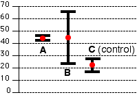
Did treatment A have a significant effect? Did treatment B?
The graph shows the mean for each data set (red dots). The dark lines represent the 95% confidence limits (± 2 standard errors).
Although both experimental means (A and B) are twice as large as the control mean, only the results in A are significant. The "true" value of B could even be simply that of the untreated animals, the controls (C).
In principle, a scientist designs an experiment to disprove, or not, that an observed effect is due to chance alone. This is called rejecting the null hypothesis.
The value p is the probability that there is no difference between the experimental and the controls; that is, that the null hypothesis is correct. So if the probability that the experimental mean differs from the control mean is greater than 0.05, then the difference is usually not considered significant. If p = <0.05, the difference is considered significant, and the null hypothesis is rejected.
In our hypothetical example, the difference between the experimental group A and the controls (C) appears to be significant; that between B and the controls does not.
| Welcome&Next Search |